Bayesian networks: From zero to working model
Over the years, we have often heard from our clients that black box machine learning solutions are unacceptable. In the previous article, we went over three key questions to ask before using a black box model, and we proposed Bayesian networks as an ideal substitute if black box models are not an option.
This article is intended to be an introduction to the world of Bayesian networks. We will start with basic Bayesian reasoning explained using a simple example. Next, we will tell you how to construct a naïve Bayes classifier using these elementary blocks. Finally, we will combine the previous steps in a full-stack Bayesian network.
Step 1: Bayesian reasoning units
Well, this chapter is a little bit technical. But don’t worry, all you need is high school math and one equation from your Statistics 101 course. This is an equation you probably know, the Bayes rule. We will use it in the so-called odds form:
Posterior odds = Prior odds × Likelihood ratio
Those words sound strange, but their meaning is straightforward:
- Prior odds – odds of an event BEFORE taking any data into account. This is something your business expert gives you.
- Posterior odds – odds of the event AFTER taking data into account. This is what you want—make prior estimates more precise.
- Likelihood ratio – this is a technical term describing how information from data affects your beliefs.
And that’s it. So far, so good. So let’s use it in this simple situation:
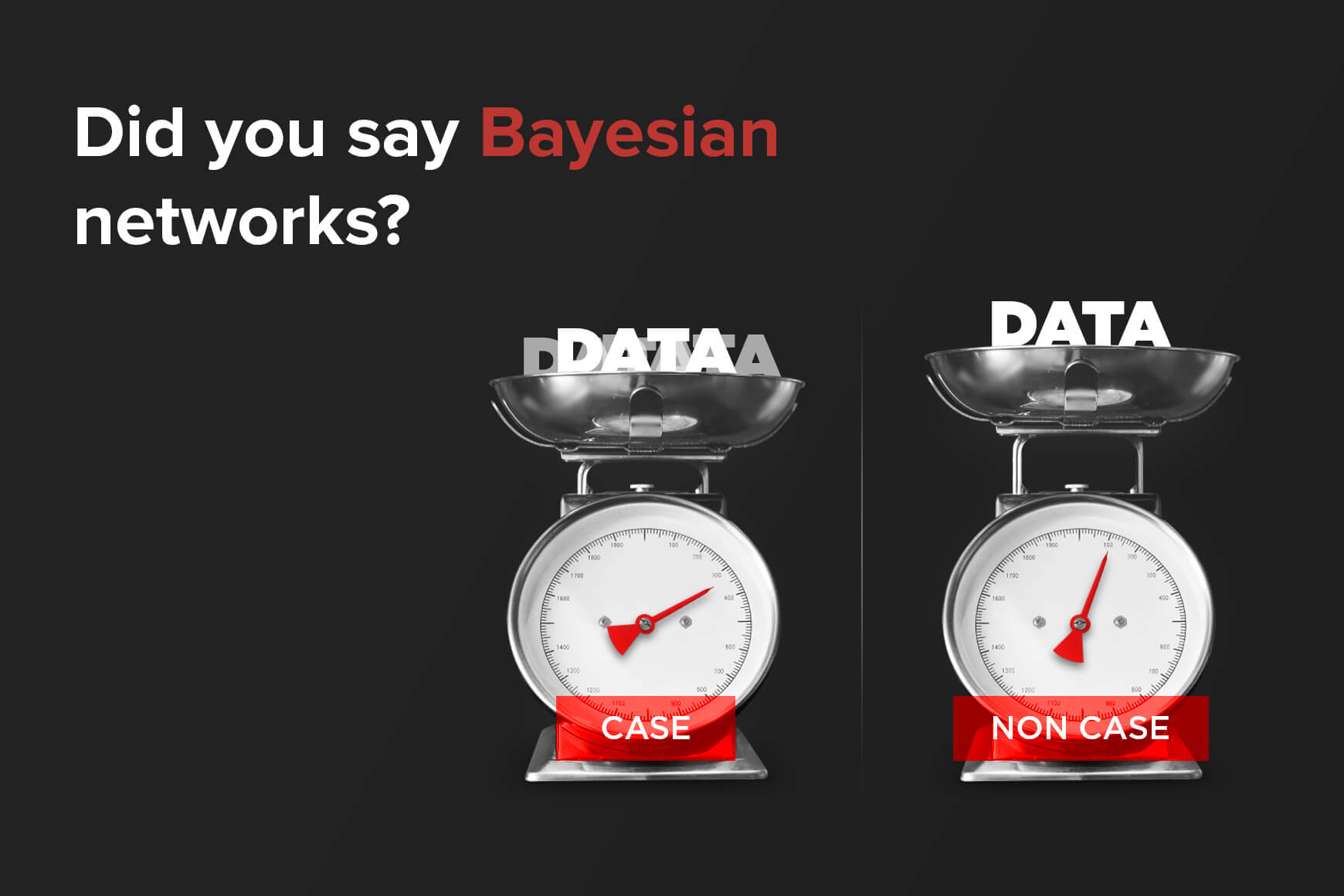
A client of our bank sent a transaction to an unknown account with the note “refrigerator”. We would like to find out whether it was a loan transfer, so we can consider offering to refinance his loan.
So, here is what we have:
- The question: What are the odds that the transaction is a loan payment?
- The evidence: The transaction note contains the word “refrigerator”.
- You get the prior odds directly from your data. That’s the ratio of loan payments to all non-loan-payment transactions your clients make.
- The posterior odds are what you want to know: How did the evidence influence your belief that the transaction is a loan payment?
- The likelihood ratio is the tricky one, and we won’t go for the mathematical explanation. Still, you will get it quite easily. Just count the occurrences of the word “refrigerator” in cases (loan payment transactions) and non-cases (other transactions). Then divide the first number by the second.
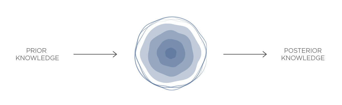
And voilà, you’ve constructed your first Bayes reasoning unit (also called a Bayesian updating step). Congratulations!
Step 2: Naïve Bayes classifiers
Of course, one piece of evidence is usually not enough. There are many attributes of a transaction that can be measured—the amount, currency, timestamp, transaction symbols, etc. Thus, you need a way to combine them.
Indeed, those Bayes reasoning units can be linked together. Then, the whole process is described in these 3 steps:
- Start with the prior odds, just as with the simple Bayes reasoning unit.
- For each piece of evidence:
- Use the odds resulting from the previous step as the prior odds.
- Process the piece of evidence the way we’ve described for the simple Bayes reasoning unit.
- The final posterior odds is your desired outcome.
That’s it. It feels just like a string of beads.

This simple yet powerful machine learning model is called a naïve Bayes classifier. As you can see, they can be computed very quickly—just multiply several numbers and you’re done. Great!
Maybe you haven’t noticed, but you use this tool daily. How is that so? For example, it’s implemented at the heart of your inbox spam filter. The shreds of evidence are words that are much more prevalent in spam than in regular emails (e.g., ‘F r e e’, ‘$$$’). And their prevalence gives you those likelihood ratios we need.
This is not the only use case for Bayes classifiers. They are used in a variety of fields—such as medicine, law (listen to this excellent talk from ScienceCafe.cz about Bayesian reasoning and forensic genetics) and sports betting. So let’s start using them in finance and banking!
Step 3: Bayesian networks
Ok, let’s step back a bit. Some assumptions have been mentioned, haven’t they? To combine Bayes reasoning units this way, you have to ensure that:
- All pieces of evidence are (conditionally) independent.
That may sound odd. Again, we won’t get into the mathematical details here, but what it means is:
- All the likelihood ratios we used to adjust our prior knowledge need to remain the same regardless of the evidence already processed.
Ok, but what does that mean?!
- Let’s say you have two pieces of evidence:
- The transaction contains “refrigerator” in the note.
- The transaction amount is greater than 3 600 € .
- Now, there is a problem:
- The likelihood ratio for the second piece of evidence is surely not the same once we know about the first piece of evidence. (Just imagine a refrigerator for that price!)
- Thus, you are not allowed to combine this information this way!
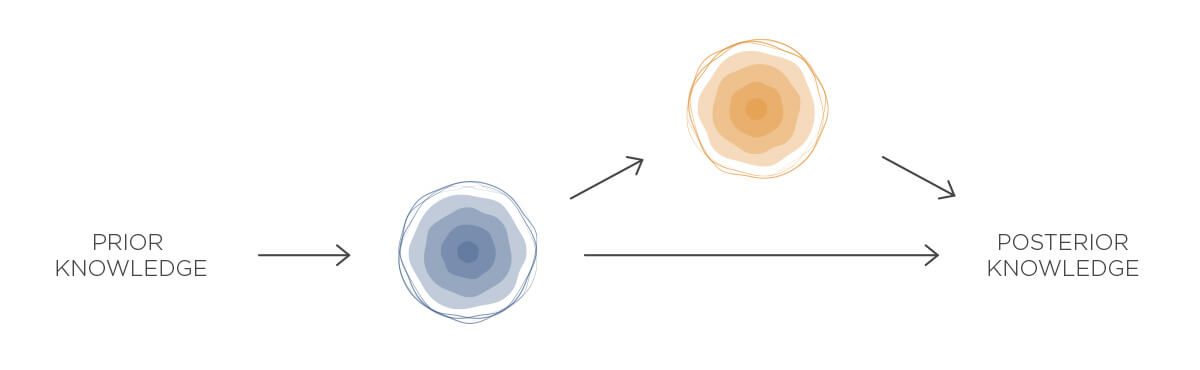
And this is where Bayesian networks come into play. You can split the reasoning conditioned on the first piece of evidence. Let’s say we take into account the second piece of evidence only if the first one is not present:
Of course, you have to build this orange Bayes reasoning unit on the corresponding subset of data. But the logic remains the same. So it’s not a big deal.
And voilà, you’ve created your very first Bayesian network! Congratulations!
Go advanced
We have just seen how to combine two pieces of evidence. Each Bayes reasoning unit now tells you two important things—how to adjust your prior knowledge (so far) and which evidence to process next. Of course, if you are combining many pieces of evidence, it can get complicated as you can see in the following example.
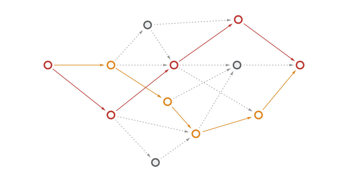
Advanced Bayesian network
But remember: the basic concept is still simple. You can imagine such a Bayesian network as a set of individual naïve Bayes classifiers. So, its outputs are both easy to get and easy to interpret! And that’s awesome.
Of course, there are many advanced ways to fine-tune your Bayesian network. You can consider more than one outgoing transaction from a client. You can add more layers reflecting different modelling levels. You can take a timestamp into account with dynamic Bayesian networks. You can use continuous variables as evidence in continuous Bayesian networks. And the list goes on.
All those advanced operations are very interesting. Some of them have already been implemented in our detectors. Unfortunately, they are way outside the scope of this article. If you are interested, let’s get in touch and discuss those exciting topics personally.